Man, I am so easily nerd-sniped. First, I can just tell that the wedding profession matcher is going to push me to dig out all sorts of weird, distinctive patterns in the pairings between professionals. But, recently, I found myself idly simulating the answer to another kind of question altogether.

The St. Petersburg Paradox

The St. Petersburg Paradox describes a game with a mathematically “infinite” expected payoff but one that definitely does not feel worth playing. The Wikipedia article is quite good on the subject, but to put it briefly here:

You start the game with two dollars. This is your ‘stake.’ Then, the casino flips a fair coin. If that coin comes up heads, then your stake is doubled. If the coin shows tails, you stop the game and win the stake as is.

Mathematically, the “expected return” of a game of chance or investment is the winnings multiplied by how like you are to win. Here, you can think of a bunch of different “win states:”

• you get tails on the first coin, with a payout of $2
• you get tails on the second coin, with a payout of $4
• you get tails on the third coin, with a payout of $8

And so on. Theoretically, if you were very lucky, this could go on for a very long time, possibly infinitely long. Thus, the expected return of the game overall is infinite:

$$ \mathbf{E}[r] = \frac{1}{2}(2) + \frac{1}{4}(4) + \frac{1}{8}(8) + \dots = 1 + 1 + … = \infty $$

The paradox comes in when trying to figure out how much you might pay to enter this game. What’s a fair price for entry? Well… your gut may be that you’re very unlikely to win anything more than eight bucks. And, you’d be right. So, you may be interested in paying less than that to break even.

So, let’s see how often you’d be right!

Simulating an Answer

To figure this out empirically, you can just simulate the outcomes of this process, and determine what you’d need to bet in these simulations to break even. Here, I’ll write the gamble using Python, and we can piece together the distribution of results.

First, we build a python function describing the game itself:

 1
 2
 3
 4
 5
 6
 7
 8
 9
10
11
12

import numpy, seaborn
from numba import njit # let's go fast 🚀

@njit
def st_petersburg(stake=2, p_heads=.5, max_iterations=1e9):
    i = 0
    while i < max_iterations:
        is_tails = numpy.random.random() > p_heads
        if is_tails:
            return stake
        stake *= 2
        i += 1

Now, to see this work:

>>> st_petersburg()
2

Oof! One game in, and we can’t even get past the first flip! Let’s try a few more times:

>>> st_petersburg()
2
>>> st_petersburg()
2
>>> st_petersburg()
8
>>> st_petersburg()
16
>>> st_petersburg()
2

OK, well, a few wins there. Let’s go all in on the simulation, and construct 10,000 realizations:

>>> winnings = [st_petersburg() for _ in range(10_000)]

So, we’ve run our simulations. What do the typical winnings look like?

Well, we can visualize them using the empirical cumulative density function, which is (in my opinion), a better way at understanding the distribution of values than a typical histogram..

>>> ax = seaborn.ecdfplot(winnings); ax.set_xlim(0,50); plt.show()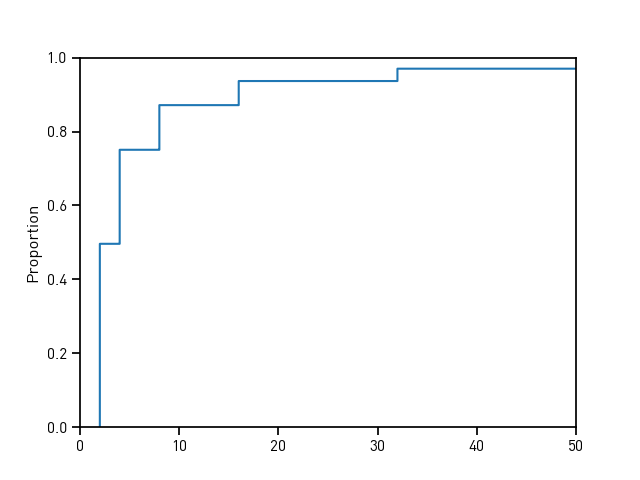

I think of this plot like this.

The line expresses the fraction of values that are at least as big as the X value. As you go from left to right, you “see” more data, and your line rises. When the line rises quickly, it means a lot of data falls in a small range of values, and when it rises slowly, it means that very few points (if any) are in that range. You can also think of the line as plotting the “percentile” of the value on the X axis; when the line passes through (11, .9), then you know that 11 is in the 90th percentile of values in your data, with 90% of the values being smaller than (or equal to) 11.

The nice thing about this plot is that we can immediately see the percent of simulations where we’d lose money. The blue line shows you the percent of simulations where you’d lose money if you paid the value on the X axis to enter the game. For example, if you paid 10 bucks to play the game, you’d only break even or profit about 12% of the time. While that seems small, the odds of winning here are quite good for the player (7ish to 1 odds to win), compared to typical casino games. But, among those games where you’d win, you’d only win a median of 6 bucks, over and above the entry fee. Moving to a $20 entry fee about halves this chance of breaking even, and doubles the median profit to 12 bucks. But, moving to a $40 halves your chances of breaking even again, but the median profit skyrockets to 88 bucks!

Of course, armed with this, you can decide how “risk tolerant” you are and find the entry price past it doesn’t make sense for you to risk playing the game.¹ So, how much would you pay to play the St. Petersburg game?