Does projection matter for compactness indices?
This is a quick and dirty exploration of the compactness impacts of changing the projection of data on compactness measures.
import geopandas as gpd
import numpy as np
import matplotlib.pyplot as plt
from compact import reock as _reock
import pysal as ps
import seaborn as sns
%matplotlib inline
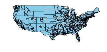
The data I’m using is the 113th districts from my Scientific Data publication, sourced originally from Jeff Lewis.
df = gpd.read_file('./districts113.shp').query('STATENAME not in ("Alaska","Hawaii")')
df.plot(color='skyblue', edgecolor='k')
plt.axis('off')
plt.show()
I’ll just check three measures, a pure area one (the convex hull areal ratio), a mixed perimeter-area one (the isoperimetric quotient), and an area-dependent one that is sensitive to the angles inherited from its planar projection (the Reock measure). The last one is notable, since its value is both dependent on the size of its minimum bounding circle, which depends on the angle preserving properties of the projection, and the accuracy of the areas of those shapes, which is not conserved by conformal projections.
def convex_hull(geom):
    return geom.area / geom.convex_hull.area
def ipq(geom):
    return (4*np.pi * geom.area) / (geom.boundary.length)**2
def reock(geom):
    return _reock(ps.cg.asShape(geom)) #custom implementation
ipq_unprojected = df.geometry.apply(ipq).values
cha_unprojected = df.geometry.apply(convex_hull).values
reock_unprojected = df.geometry.apply(reock).values #takes a while to solve mbc in pure python
df.crs = {'init':'epsg:4269'}
albers_eac = df.copy(deep=True).to_crs(crs='+proj=aea +lat_1=20 +lat_2=60 +lat_0=40 +lon_0=-96 +x_0=0 +y_0=0 +datum=NAD83 +units=m +no_defs')
lambert_cc = df.copy(deep=True).to_crs(crs='+proj=lcc +lat_1=20 +lat_2=60 +lat_0=40 +lon_0=-96 +x_0=0 +y_0=0 +datum=NAD83 +units=m +no_defs')
webmerc_ccyl = df.copy(deep=True).to_crs(crs='+proj=merc +a=6378137 +b=6378137 +lat_ts=0.0 +lon_0=0.0 +x_0=0.0 +y_0=0 +k=1.0 +units=m +nadgrids=@null +wktext  +no_defs')
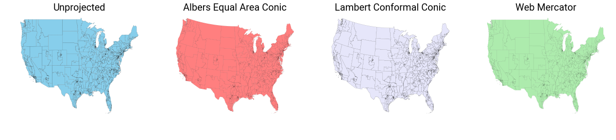
Visually, you can tell that something changes when you use the conic projections with preserving properties. But, the real differences are conceptual, in that the various projections will result in strongly different area, angle, and length computations for the shapes involved.
f,ax = plt.subplots(1,4,figsize=(22,4))
df.plot(color='skyblue', linewidth=.1, ax=ax[0], edgecolor='k')
albers_eac.plot(color='red', linewidth=.1, alpha=.5, ax=ax[1], edgecolor='k')
lambert_cc.plot(color='lavender', linewidth=.1, ax=ax[2], alpha=1, edgecolor='k')
webmerc_ccyl.plot(color='limegreen', linewidth=.1, ax=ax[3], alpha=.4, edgecolor='k')
[_ax.axis('off') for _ax in ax]
[ax[i].set_title(['Unprojected',
                  'Albers Equal Area Conic',
                  'Lambert Conformal Conic',
                  'Web Mercator'][i], fontsize=20)  for i in range(4)]
plt.show()
Now, we can compute the three measures for each of the three projections:
cha_ea = albers_eac.geometry.apply(convex_hull).values
cha_cc = lambert_cc.geometry.apply(convex_hull).values
ipq_ea = albers_eac.geometry.apply(ipq).values
ipq_cc = lambert_cc.geometry.apply(ipq).values
reock_ea = albers_eac.geometry.apply(reock).values
reock_cc = lambert_cc.geometry.apply(reock).values
cha_mcyl = webmerc_ccyl.geometry.apply(convex_hull).values
ipq_mcyl = webmerc_ccyl.geometry.apply(ipq).values
reock_mcyl = webmerc_ccyl.geometry.apply(reock).values
from scipy import stats as st
unprojected = [cha_unprojected, ipq_unprojected, reock_unprojected]
aeas = [cha_ea, ipq_ea, reock_ea]
lccs = [cha_cc, ipq_cc, reock_cc]
mcyl = [cha_mcyl, ipq_mcyl, reock_mcyl]
I’ll compute their correlations in terms of both linear association and rank association.
Personally, I’m more concerned about their rank association.
pearsons = [[st.pearsonr(proj,unproj) for proj,unproj in zip(unprojected, aeas)],
            [st.pearsonr(proj,unproj) for proj,unproj in zip(unprojected, lccs)],
            [[st.pearsonr(proj,unproj) for proj,unproj in zip(unprojected, mcyl)]]]
kendalls = [[st.kendalltau(proj,unproj) for proj,unproj in zip(unprojected, aeas)],
            [st.kendalltau(proj,unproj) for proj,unproj in zip(unprojected, lccs)],
            [[st.kendalltau(proj,unproj) for proj,unproj in zip(unprojected, mcyl)]]]
proj_titles = ['Unprojected', 'Albers EA', 'Lambert EC', 'Web Mercator']
measures = ['Convex Hull', 'IPQ', 'Reock']
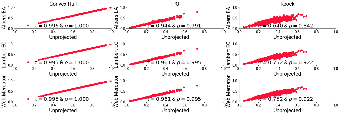
And, I’ll plot the comparisons with the unprojected measure on the X axis and the projections on the Y axis, with each comparison projection having its own row.
You’ll see that, for most of the measures, the differences due to projection are quite minor. However, in all cases, the change of the Kendall’s Tau mean that, in all cases, some districts become relatively more- or less-compact than others; they jockey for position.
This degrades exessively in the case of the reock measure. In this case, both the projections have a significant change in the resulting metric depending on whether a projection is used.
f,ax = plt.subplots(3,3,figsize=(18,6), sharex=True, sharey='col')
ax[0,0].scatter(cha_unprojected, cha_ea)
ax[0,0].text(s='$\\tau={:.3f}$ & $\\rho = {:.3f}$'.format(kendalls[0][0].correlation, pearsons[0][0][0]),
             x=.2, y=.05, fontsize=20)
ax[0,1].scatter(ipq_unprojected, ipq_ea)
ax[0,1].text(s='$\\tau= {:.3f}$ & $\\rho = {:.3f}$'.format(kendalls[0][1].correlation, pearsons[0][1][0]),
             x=.2, y=.05, fontsize=20)
ax[0,2].scatter(reock_unprojected, reock_ea)
ax[0,2].text(s='$\\tau= {:.3f}$ & $\\rho = {:.3f}$'.format(kendalls[0][2].correlation, pearsons[0][2][0]),
             x=.2, y=.05, fontsize=20)
ax[1,0].scatter(cha_unprojected, cha_cc)
ax[1,0].text(s='$\\tau= {:.3f}$ & $\\rho = {:.3f}$'.format(kendalls[1][0].correlation, pearsons[1][0][0]),
             x=.2, y=.05, fontsize=20)
ax[1,1].scatter(ipq_unprojected, ipq_cc)
ax[1,1].text(s='$\\tau= {:.3f}$ & $\\rho = {:.3f}$'.format(kendalls[1][1].correlation, pearsons[1][1][0]),
             x=.2, y=.05, fontsize=20)
ax[1,2].scatter(reock_unprojected, reock_cc)
ax[1,2].text(s='$\\tau= {:.3f}$ & $\\rho = {:.3f}$'.format(kendalls[1][2].correlation, pearsons[1][2][0]),
             x=.2, y=.05, fontsize=20)
ax[2,0].scatter(cha_unprojected, cha_cc)
ax[2,0].text(s='$\\tau= {:.3f}$ & $\\rho = {:.3f}$'.format(kendalls[1][0].correlation, pearsons[1][0][0]),
             x=.2, y=.05, fontsize=20)
ax[2,1].scatter(ipq_unprojected, ipq_cc)
ax[2,1].text(s='$\\tau= {:.3f}$ & $\\rho = {:.3f}$'.format(kendalls[1][1].correlation, pearsons[1][1][0]),
             x=.2, y=.05, fontsize=20)
ax[2,2].scatter(reock_unprojected, reock_cc)
ax[2,2].text(s='$\\tau= {:.3f}$ & $\\rho = {:.3f}$'.format(kendalls[1][2].correlation, pearsons[1][2][0]),
             x=.2, y=.05, fontsize=20)
for i,row in enumerate(ax):
    for j,ax_ in enumerate(row):
        ax_.set_ylim(0,1)
        ax_.set_xlim(0,1)
        sns.despine(ax=ax_)
        if i == 0:
            ax_.set_title(measures[j], fontsize=20)
        ax_.set_ylabel(proj_titles[i+1], fontsize=20)
        ax_.set_xlabel(proj_titles[0], fontsize=20)
f.tight_layout(pad=.1)
plt.show()
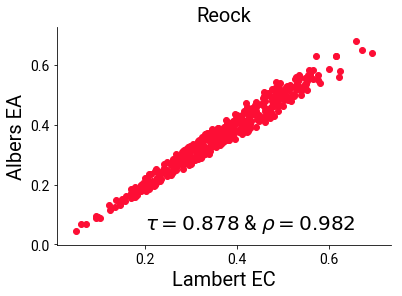
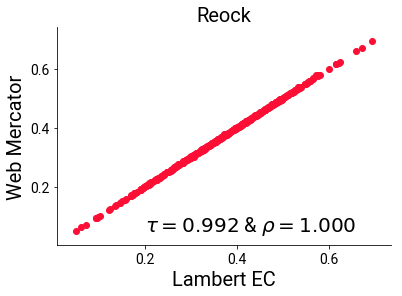
Critically, the projected versions themselves agree much more strongly on the reock measure than they do with the unprojected measure, with their rank and linear correlations maintaining a healthy association:
plt.scatter(reock_cc, reock_ea)
plt.text(s='$\\tau= {:.3f}$ & $\\rho = {:.3f}$'.format(st.kendalltau(reock_cc, reock_ea)[0],
                                                       st.pearsonr(reock_cc, reock_ea)[0]),
             x=.2, y=.05, fontsize=20)
sns.despine()
plt.xlabel("Lambert EC", fontsize=20)
plt.ylabel("Albers EA", fontsize=20)
plt.title("Reock", fontsize=20)
plt.show()
plt.scatter(reock_cc, reock_mcyl)
plt.text(s='$\\tau= {:.3f}$ & $\\rho = {:.3f}$'.format(st.kendalltau(reock_cc, reock_mcyl)[0],
                                                       st.pearsonr(reock_cc, reock_mcyl)[0]),
             x=.2, y=.05, fontsize=20)
sns.despine()
plt.xlabel("Lambert EC", fontsize=20)
plt.ylabel("Web Mercator", fontsize=20)
plt.title("Reock", fontsize=20)
plt.show()
So, does it matter?
Probably not, especially at the state level, considering how strong these correlations are. However, if we were concerned with particularly pathological district shapes, we need to use the correct relevant projections.
Sometimes, this will be impossible, since all projections trade off accuracy in some way. But, practically speaking, these tradeoffs (at the state level) are more precise than relevant to the computation of the statistic itself.